
8 | India Seen Through First Synchronous Census of 1881: A Demographic Overview
- Apr 10
- 12 min read
Updated: 3 days ago
By Shivakumar Jolad, Siddharth Ramkumar, Gaurav Kalyani and Kriti Bhargava
Published on: 5 May 2026
Introduction
As the first synchronous census, the 1881 census represented a landmark operation that systematically recorded demographic and social data across every district and province in colonial India. It provided a first ever liable quantitative snapshot of India in the demographic history. Conducted across vast and diverse territory, this census exercise generated a wealth of data that shaped how the colonial state would understand and govern India, as well as how subsequent scholars understand the demography and socio-economic life of people in that era.
While previous counts were localized or staggered, this operation captured a total population of 254 million within a single administrative frame, exposing an empire defined by extreme regional contrasts and deep structural fragilities. It revealed a demographic regime characterized by prevalence of youth, stark contrasts and a population trapped in recurrent crises. The census recorded a society where growth in prosperous years was frequently wiped out by the demographic shocks of famine and epidemic disease.
Going beyond just a head-count, the 1881 census established an essential benchmark for modern demographic reconstructions. It brought to light critical data points on sex ratios, civil conditions and population demographics across a vast territory, providing the colonial state with its first comprehensive picture of the carrying capacity of the land. This article explores the key findings of this massive demographic exercise.
Population, Population Density, and Regional Contrasts
The Census 1881 gave the first comprehensive picture of population and its distribution across all provinces and territories, and territories across British India. As discussed in the previous article, the coverage was much wider and more accurate (especially enumeration of women and children), Note that Burmah (Burma) was also part of the British Indian administration. The total population of British India , including Burma was at 254 million (Plowden, 1883).
A few large provinces dominated. Bengal (with ~69.5 million people) alone accounts for over a quarter of the population, followed by North-Western Provinces (~44.1 million) and Madras (~31.2 million) follow. Bengal (it includes present day West Bengal, Bihar, Orissa, and Bangladesh) was also the largest in Area at 193,198 square miles. This was followed by Madras (141,000 sq miles) , Rajputana (princely states) and Bombay province. Bombay also included Sindh till 1931 (Plowden, 1883).
After the top 3–4 regions, population drops sharply—most other provinces and princely regions are below 20 million, many below 5 million. Coorg and Ajmer were minor provinces, which were later administered as Chief commissioners province. Feudatory (princely) states were generally much smaller in population compared to British-administered provinces. Hyderabad was the largest state with 9.85 million inhabitants and 81,800 square miles (Plowden, 1883).
Population Density: The final results showed an average population density of 184 persons per square mile for the entire Indian Empire (Plowden, 1883). This average, however, was merely an arithmetical expression that masked extreme regional contrasts dictated by rainfall, soil quality, and historical political conditions (Gait, 1912). The most striking contrast was between the Bengal Presidency, with a density of 360 persons per square mile — nearly half as high again as Italy's 249 — and the province of Burma, with only 43 persons per square mile, dropping to just six in the Salween division (Plowden, 1883). Both Burma and Rajputana states had substantial areas but relatively lower population density.
These variations were largely attributed to soil quality and water supply; the Gangetic plain provided level alluvium where practically every inch was cultivable, while areas like Rajputana and Baluchistan suffered from scanty rainfall where little cultivation was possible without irrigation (Gait, 1912).
Table: Population Density Comparisons, Census of India 1881. Source: Report on the Census of British India, 1881, pp. 7–8.
Region / Country | Population Density (per sq. mile) | Note |
Bengal (India) | 360 | Most populous province |
Italy (European comparison) | 249 | Reference benchmark |
All-India Average | 184 | Official census figure |
Burma (India) | 43 | Least dense province |
Salween Division (Burma) | 6 | Extreme sparsity |
Howrah district (Bengal) | 1,335 | Highest recorded density |
Benares district | 894 | Dense Gangetic plain |
Patna district | 845 | Dense Gangetic plain |

At the district level, the census identified thirteen districts in Bengal and the North-West Provinces where density consistently exceeded 700 persons per square mile (Plowden, 1883).
The highest recorded density was in Howrah at 1,335 persons per square mile, followed by Benares (894), Sarun (870), and Patna (845) (Plowden, 1883). Collectively, these thirteen districts supported over 20 million people in an area only half the size of England.
Administrators used these density figures to analyze the carrying capacity of the land, noting that in many parts of Upper India, the limit in this respect has almost been reached under existing agricultural conditions (Plowden, 1883). This foundational analysis would go on to shape British policies regarding famine relief and internal migration for the remainder of the century (Dyson, 2022).
Urban vs. Rural Structure
The population was roughly 91% rural and 9% urban. In rural areas, the village hierarchy was self-sufficing, with established roles for headmen, accountants, and artisans (smiths, weavers, potters) to serve the immediate needs of cultivators. Large-scale factory industry was mostly confined to cities like Bombay, where approximately 36,000 people (9.5% of the working community) were employed as mill hands (Plowden, 1883).
Table: Percentage and Number of Urban and Rural Population
This table details the distribution of the population between villages (rural) and towns (urban) across various provinces and states.

Table: Population of the Great Cities of India
The following cities were identified as the largest in the Empire
Cities | Population |
Bombay | 772,196 |
Calcutta | 766,298 |
Madras | 405,848 |
Hyderabad (with Secunderabad) | 354,962 |
Lucknow | 261,303 |
Benares | 199,700 |
Delhi | 173,393 |
Patna | 170,654 |
Agra | 160,203 |
Bangalore | 155,857 |
Amritsar | 151,896 |
Cawnpore | 151,444 |
Lahore | 149,369 |
Allahabad | 148,547 |
Jeypore | 142,578 |
Rangoon | 134,176 |
Poona | 129,751 |
Ahmedabad | 127,621 |
Bareilly | 113,417 |
Surat | 109,844 |
Howrah | 105,206 |
Baroda | 101,818 |

The distribution of settlements in 1881 India shows a clear gradient from highly dispersed to more nucleated habitation patterns across provinces. A large share of regions—particularly the feudatory areas of Central Provinces, Punjab, and North-Western Provinces—are dominated by very small villages (under 200 population), indicating fragmented agrarian landscapes and likely subsistence-oriented rural economies. Moving across the spectrum, provinces such as Bengal, Burma, Mysore, and the Central Provinces (British) display a more balanced mix of small and mid-sized villages, suggesting transitional settlement systems.
At the other end, western and southern regions like Bombay, Baroda, Travancore, and especially Cochin exhibit a relatively higher proportion of larger settlements (500+ and 1000+), pointing toward more clustered habitation, possibly linked to stronger market integration, irrigation networks, or administrative consolidation. The “All India” average, placed at the end, reinforces that while small villages predominate nationally, there exists substantial regional variation in settlement structure shaped by ecological, economic, and historical factors.
Growth Trends, Famine, and the Demographic Crisis
Between 1871 and 1921, the population of India grew from approximately 255 million to 305 million, implying a very low average annual growth rate of just 0.36% (Dyson, 2018).
Mortality during this period was also linked to epidemic disease. In the Deccan famine (discussed at length in the previous article), outright starvation was often secondary to outbreaks of cholera and malaria (Dyson, 2018). Estimates of excess deaths for the 1876–78 famine range from official figures of 5.6 million to unofficial assessments as high as 9.4 million (Dyson, 2018).
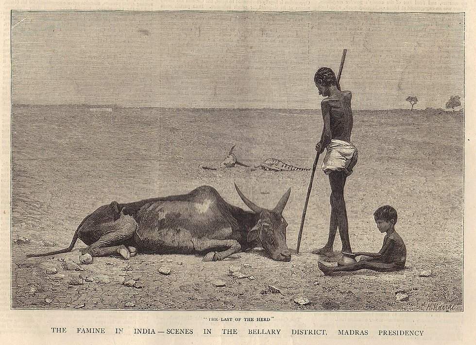
The 1881 data confirmed that these deaths fell hardest on the labourers, the poorer and the lower agricultural people in rural districts who lived on the bare margin of subsistence (Plowden, 1883).
Coupled with life expectancies hovering between 22 and 27 years, the census captured a population trapped in a pattern of recurrent crisis where any growth in prosperous years was repeatedly wiped out by such demographic shocks (Dyson, 2018).

Age Structure and Life Expectancy
The age structure of India's population in 1881 was fundamentally characterized by extreme youth, reflecting uncontrolled fertility and high mortality. The Census recorded that 38.9 per cent of the inhabitants were aged 0–14 years, whereas only 5.9 per cent survived to the age of 60 and over (Dyson, 2018).
This ‘superabundance’ of the young was noted as a distinguishing feature of Indian society, where the aged are rare . The average life expectancy at birth was estimated at just 23.5 years, compared to nearly 40 years in England (Dyson 2018; Plowden, 1883).


Infant mortality was the primary driver of these low figures; G. F. Hardy deduced that nearly 40 per cent of all babies died before attaining their fifth birthday (Dyson, 2023; Plowden, 1883).
Despite the extreme irregularity of age reporting — including a strong tendency for respondents to guess their ages or select round numbers like 20, 30, and 40 — the 1881 data became the essential benchmark for modern demographic reconstruction in India (Plowden, 1883; Maheshwari, 1996).
Because vital registration was virtually useless at the time, later demographers used the 1881 age returns to estimate fertility and mortality patterns by analyzing the survivorship of population age groups from one census to the next (Dyson, 2018; Dyson, 2022).
These methods allowed researchers to identify female age shifting and other systematic errors, providing the first reliable quantitative snapshot of India's pre-transitional demographic history (Dyson, 2022).
Sex Ratio and Gender Imbalance
The 1881 Census brought to light early signs of gender imbalance, recording 129,941,851 males and 123,949,970 females, a sex ratio of approximately 105 males per 100 females.
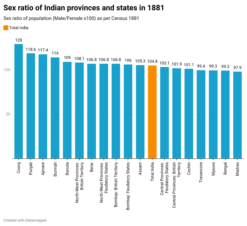
Strong male bias could be seen in Punjab (especially British territory), North West Provinces (UP), Rajputana, and Berar (Central India). It indicates significant gender imbalance, possibly linked to social structure, enumeration biases, or migration patterns. Government documents observed that many census workers failed to recognize that the enumeration of women was a necessary part of the process (Plowden, 1883).
This was attributed to the low value placed on women in society and the cultural tendency to keep information about female members private. Marriageable girls between the ages of 10 and 20 were systematically concealed by householders operating under false shame among the upper classes (Plowden, 1883).
As a comparison we can study the sex ratio in European population , which shows far greater degree of evenness ~50
Table: Proportion of the Sexes in different European States (p. 52) | |||||
States | Year of Census | Total Population | Males | Females | Sex ratio (M/F) × 100 |
Germany | 1880 | 45,234,061 | 22,185,433 | 23,048,628 | 96.25 |
England and Wales | 1881 | 25,974,439 | 12,639,902 | 13,334,537 | 94.79 |
Hungary | 1880 | 15,625,152 | 7,695,533 | 7,929,619 | 97.05 |
Denmark | 1880 | 1,980,259 | 972,832 | 1,007,427 | 96.57 |
Sweden | 1880 | 3,875,237 | 1,901,820 | 1,973,417 | 96.37 |
Switzerland | 1880 | 2,846,102 | 1,394,626 | 1,451,476 | 96.08 |
Netherlands | 1879 | 4,012,693 | 1,983,164 | 2,029,529 | 97.72 |
Norway | 1875 | 1,802,172 | 872,151 | 930,021 | 93.78 |
Spain | 1877 | 16,731,570 | 8,244,978 | 8,486,592 | 97.15 |
Italy | 1871 | 26,801,154 | 13,472,262 | 13,328,892 | 101.08 |
Greece | 1879 | 1,653,767 | 855,249 | 798,518 | 107.10 |
Table: Sex Ratio of the Child Population
The following table illustrates the sex ratio for child population 0-4 years, calculated in two ways (Females per 1000 Males and no of Males per 100 Females. The regions Ajmere (107.5), Punjab (Feudatory) (107.5), Punjab (British) (105.5), and N.W. Provinces (Feudatory) (101.2) show early male excess.
Province or State | Females per 1,000 Males (0–4) | Sex Ratio (M/F × 100) |
Ajmere | 930 | 107.53 |
Punjab (Feudatory States) | 930 | 107.53 |
Punjab (British Territory) | 948 | 105.49 |
North-West Provinces (Feudatory States) | 988 | 101.21 |
Burmah | 1,003 | 99.7 |
North-West Provinces (British Territory) | 1,005 | 99.5 |
Baroda | 1,020 | 98.04 |
Bombay (Feudatory States) | 1,021 | 97.94 |
Bombay (British Territory) | 1,024 | 97.66 |
Coorg | 1,040 | 96.15 |
Assam | 1,048 | 95.42 |
Hyderabad | 1,050 | 95.24 |
Central Provinces (British Territory) | 1,054 | 94.88 |
Berar | 1,055 | 94.79 |
Madras | 1,057 | 94.61 |
Bengal | 1,065 | 93.9 |
Mysore | 1,076 | 92.94 |
Central Provinces (Feudatory States) | 1,103 | 90.66 |
All India | 1,034 | 96.71 |
Source: Plowden, 1883
Marital Status
Marriage for women is a short-lived phase in a longer trajectory of widowhood
The 1881 census data on civil condition reveals a society where marriage was nearly universal and typically contracted at a very early age, creating a demographic profile fundamentally different from contemporaneous European nations (Plowden, 1883). Across the major provinces, the proportion of married females averaged 490 per 1,000, significantly exceeding the European average of approximately 330 per 1,000 (Plowden, 1883). This regime of early marriage, combined with strong social and religious prohibitions against widow remarriage, resulted in an exceptionally high prevalence of widowhood (Plowden, 1883).
More than one-fifth of the female population in Bengal (21.2%) and Mysore (25.1%) consisted of widows, a proportion more than double the highest rates recorded in Europe at the time (Plowden, 1883).
These statistics underscore how cultural institutions such as child marriage directly shaped India's population structure, contributing to a high pressure demographic regime characterized by high birth rates and the existence of a large class of female ‘despised drudges’ who remained single after the death of a spouse (Plowden, 1883).
Distribution of Marital Status by Age Group (per 1,000) | ||||
Age Group | Sex | Bengal (S / M / W) | N.W. Provinces (BT) (S / M / W) | Punjab (BT) (S / M / W) |
20–24 | Male | 300 / 677 / 23 | 302 / 675 / 23 | 435 / 544 / 21 |
Female | 15 / 887 / 98 | 35 / 937 / 28 | 49 / 923 / 28 | |
30–39 | Male | 51 / 902 / 47 | 87 / 836 / 77 | 141 / 790 / 69 |
Female | 6 / 724 / 270 | 8 / 825 / 167 | 8 / 843 / 149 | |
40–49 | Male | 23 / 899 / 78 | 58 / 825 / 117 | 91 / 786 / 123 |
Female | 4 / 500 / 496 | 6 / 627 / 367 | 6 / 664 / 330 | |
50–59 | Male | 17 / 855 / 128 | 51 / 758 / 191 | 76 / 728 / 196 |
Female | 4 / 315 / 681 | 5 / 391 / 604 | 5 / 457 / 538 | |
60+ | Male | 4 / 753 / 243 | 46 / 628 / 326 | 67 / 603 / 330 |
Female | 2 / 134 / 864 | 5 / 168 / 827 | 4 / 215 / 781 | |
Note: S = Single, M = Married, W = Widowed (per 1,000 persons)BT: British TerritorySource: Plowden (1883)m, p. 93 | ||||


Across all major religious groups in the 1881 Census, a remarkably consistent life-cycle pattern emerges. For women, marriage occurs early and rapidly—often becoming the dominant status by ages 15–19—followed by a steady and dramatic transition into widowhood. By ages 50–59 and especially 60+, widowhood overwhelmingly dominates the female population. In contrast, men exhibit a very different trajectory: entry into marriage is slower, but once married, they largely remain so throughout life, with widowhood rising only gradually and never overtaking marriage.
Religious differences primarily affect the timing of these transitions rather than their underlying structure. Groups such as Hindoo and Mahammedan populations show earlier female marriage, while Christian and Aboriginal groups display relatively delayed entry. However, the broader institutional pattern—a gendered asymmetry where women move from marriage into prolonged widowhood while men remain predominantly married—remains strikingly uniform. This suggests that what appears as religious variation is, in fact, a shared demographic regime shaped by deeper social norms around marriage, mortality, and remarriage.
Child marriage
The practice of child marriage in India around the 1881 census was nearly universal, compared to european standards. Among Hindus across the subcontinent, approximately 292 boys and nearly 860 girls in every 1000 children aged 0-9 were married (Plowden, 1881).
The census also noted that for a large proportion of these marriages, the bethrotal ceremony was observed, making it legally binding even though cohabitation did not begin until puberty. In Baroda, census reports noted some communities like Kaidva Kunbis practiced mass marriage season every 10-12 years. In the 1880 season, it was noted that parents married off babies even under the age of 1, to avoid missing the auspicious time window (Plowden, 1881).
Female children were married off significantly earlier than males. By the age of 20, only 0.85% Hindu women remained single. Pattern of child marriage was heavily influenced by religious doctrine. Hindu and Jain religions showed high frequency, followed by Muslim, where child marriage was less common. Buddhists and Aboriginal were noted to shun child marriage and it was described as ‘practically unknown’ within these groups (Plowden, 1881).
The combination of early marriage and vast difference in the age between the husband and wife created a unique demographic crisis. Because the hindu customs disallowed widow remarriage, child marriage directly resulted in ‘super abandance of widows’, many of whom were still children. Child marriage was most prevelant in Berar, followed by Hyderabad, Bengal and North-West Provinces (Plowden, 1881).
Table: Percentage of Civil Condition by Age and Religion (1881) | ||||||
Religion | Condition | 0–9 M | 0–9 F | 10–14 M | 10–14 F | 15–19 M |
Hindoo | Married | 2.96 | 8.7 | 17.55 | 53.26 | 39.52 |
Widowed | 0.1 | 0.29 | 0.63 | 2.11 | 1.57 | |
Mahammedan | Married | 0.94 | 4.93 | 9.05 | 47.04 | 30.61 |
Widowed | 0.02 | 0.2 | 0.29 | 1.29 | 0.98 | |
Aboriginal | Married | 0.95 | 1.79 | 7.96 | 22.74 | 33.03 |
Widowed | 0.03 | 0.09 | 0.17 | 0.55 | 0.91 | |
Buddhist | Married | 0.01 | 0.04 | 0.15 | 1.02 | 5.83 |
Widowed | — | — | 0.01 | 0.05 | 0.31 | |
Christian | Married | 0.34 | 0.73 | 1.39 | 9.73 | 9.96 |
Widowed | 0.01 | 0.06 | 0.05 | 0.33 | 0.23 | |
Sikh | Married | 0.74 | 2.21 | 12.33 | 36.76 | 35.15 |
Widowed | 0.02 | 0.04 | 0.23 | 0.53 | 0.96 | |
Jain | Married | 1.05 | 6.5 | 14.57 | 46.86 | 41.69 |
Widowed | 0.06 | 0.21 | 0.57 | 1.74 | 1.43 | |
Satnami | Married | 6.82 | 13.01 | 43.46 | 77.44 | 77.11 |
Widowed | 0.11 | 0.19 | 0.68 | 0.84 | 1.25 | |
Kabirpanthi | Married | 4.07 | 8.59 | 28.78 | 59.99 | 61.56 |
Widowed | 0.07 | 0.16 | 0.53 | 0.82 | 1.72 | |
Nat Worship | Married | — | — | 0.08 | 0.82 | 7.64 |
Widowed | — | — | 0.01 | — | 0.37 | |
Conclusion
The 1881 Census of India was a foundational moment in the history of modern South Asia. It created, for the first time, a coherent statistical representation of the subcontinent's population, establishing the methodological and institutional frameworks that would govern demographic analysis of India for the following century. Its achievement of synchronous, all-India enumeration marked the emergence of a fundamentally new relationship between the colonial state and the population it governed.
In the phrase of one demographic historian, the 1881 census was the moment when "suddenly a massive amount of demographic and other evidence" became available from which scholars could begin to reconstruct the population history of the subcontinent (Dyson, 2018).
Since 1881, as Gait noted, "a general synchronous census has been taken every ten years." This regularization transformed total visibility from a one-time aspiration into a continuous, decennial system of governance and knowledge production; one whose categories, methods, and assumptions were laid down in the cold February of 1881 and whose consequences extended far beyond the empire that created them.
(Authors: Dr. Shivakumar Jolad works as Associate Professor (Public Policy), and is the Chair of Center for Legislative Education and Research and Director India State Stories, FLAME University, Pune;
Siddharth Ramkumar is an undergraduate student at FLAME University;
Gaurav Kalyani works as Research Associate at the Center for Legislative Education and Research, FLAME University, Pune;
Kriti Bhargava is an undergraduate student at FLAME University
Shivakumar and Siddharth did research and primary writing; Kriti contributed to research and writing; Gaurav and Shivakumar contributed to conceptualization, research and editing)
References
Bhagat, R. B. (2006). Census and caste enumeration: British legacy and contemporary practice in India. Genus, 62(2), 119–134. http://www.jstor.org/stable/29789312
Dyson, T. (2018). A population history of India : from the first modern people to the present day. Oxford University Press.
Dyson, T. (2022). India’s Historical Demography: Studies in Famine, Disease and Society. Routledge.
Gait, E. A. (1912). The Indian Census. Journal of the Royal Society of Arts. http://www.jstor.org/stable/41340101
Gill, M. S. (2007). Politics of population census data in India. Economic and Political Weekly, 42(3), 241–249.
Maheshwari, S. (1996). The census administration under the raj and after. Concept Pub. Co.
Plowden, W.C ( 1883 ). Report on the Census of British India taken on the 17th
February 1881, London, Eyre and Spottiswoode.


Comments