13 | Demographic Overview of Indian Subcontinent in General Report of 1891 Census

By Umesh Bedkute and Shivakumar Jolad

Published on: 11 June 2026

Introduction

The second general Census of India, conducted on the night of 26 February 1891, offers a detailed picture of India at the end of the nineteenth century. Baines described India as being more like a continent than a single country because of its vast size and diversity. Covering nearly one-fifth of the world’s population at the time, the census provides valuable insights into demographic trends, social customs, and the expanding reach of colonial administration. This article examines the major findings of the 1891 Census, including population growth, population density, sex ratios, and the distribution of religious communities across British provinces and the Feudatory States.

National Population and Decadal Change

The 1891 Census recorded a total population of 287.2 million people, up from 253.8 million in 1881. In areas that were counted in both censuses, the population increased by nearly 27.8 million people over the decade, representing a growth rate of 10.96 percent. Population growth was uneven across regions, with the British Provinces recording an increase of 9.7 percent, while the Feudatory States experienced a much higher growth rate of 15.5 percent.

Baines pointed out that although the increase of nearly 28 million people was enormous in absolute terms, greater than the entire population of England at the time, the rate of growth was relatively modest compared with rapidly growing colonies such as New South Wales and Victoria.

Population by Provinces and Feudatory States

The population of India was administratively divided between the British Provinces, which contained about 77 percent of the population, and the Feudatory States, which accounted for the remaining 23 percent.

Among the British Provinces, Bengal [which included West Bengal, Bangladesh, Bihar, Jharkhand and British districts of Orissa] remained the most populous, with 71,346,987 inhabitants. Its population was nearly equal to the combined populations of the United States and Mexico in 1890. Madras ranked second with 35,630,440 people, a figure comparable to the population of the United Kingdom or Austria-Hungary at the time. 

The North-Western Provinces, with 34,251,251 inhabitants, and Oudh, with 12,650,831, together supported a population almost as large as that of the entire German Empire. Panjab recorded a population of 20,866,847, while Bombay, excluding Sindh, had 15,985,270 inhabitants.

The Feudatory States together had a population of more than 66 million people and occupied a vast territory. 

Among these states, Hyderabad was the largest, with a population of 11,537,040, making it nearly as populous as England and Scotland combined. Rajputana, with 12,016,102 inhabitants, and Central India, with 10,318,812, together occupied an area comparable to that of the German Empire. Mysore recorded a population of 4,943,604, which was larger than the population of Portugal despite covering a much smaller area.

Population Density Across Provinces

The average population density for India in 1891 was 184 persons per square mile (which equals 71.04 persons per square kilometer;  As per the official 2011 Census of India, the national population density was 382 persons per square kilometre)  However, this national figure concealed major regional differences. Population density was much higher in the British Provinces, where it averaged 230 persons per square mile, than in the Feudatory States, where the average was only 111.

Among the provinces, Oudh was the most densely populated, with 522 persons per square mile, followed by Bengal with 471. At the other end of the spectrum were the frontier and desert regions. Upper Burma recorded only 35 persons per square mile, while Sindh had a density of 60.

The highest concentrations of population were found in the Gangetic Valley and the delta regions. Some rural districts were especially crowded; for example, the Sáran district in Bengal had a density of 930 persons per square mile. These densely settled areas were supported largely by intensive agriculture, particularly rice cultivation on fertile alluvial soils. Among the Feudatory States, Baroda was the most densely populated, with 294 persons per square mile, while the mountainous state of Kashmir was among the least densely populated, with only 31 persons per square mile.

Population density in colonial India displayed striking regional contrasts. The most densely populated provinces were concentrated in the fertile Indo-Gangetic plain, with Oudh (522 persons per square mile), Bengal (471), and the North-West Provinces (411) recording densities far above the British Indian average of 230 persons per square mile. At the district level, Saran in Bengal emerged as the most densely settled district in British India with 930 persons per square mile, closely followed by Benares (914) and Lucknow (800).

In contrast, the sparsest regions were located in frontier, forested, and desert tracts. Upper Chindwin in Upper Burma had only four persons per square mile, while the Chittagong Hill Tracts (20), Thar and Parkar in Sindh (23), and the remote hill regions of Assam also remained thinly populated. Among the princely states, population density ranged from the relatively dense Madras States (385) and Baroda (294) to the sparsely populated territories of Kashmir (31) and Rajputana (92). The contrast between Saran and Upper Chindwin—a ratio exceeding 230 to 1—highlights the extraordinary demographic diversity that characterized late nineteenth-century India.

Population Change 

Over the decade between the 1881 and 1891 censuses, India experienced substantial population growth, reversing the population stagnation and decline associated with the famine-stricken 1870s. Baines distinguished between genuine demographic growth and increases arising from improved census coverage and administration. The 1891 Census recorded a total population of 287.2 million, compared to 253.8 million in 1881. Restricting the comparison to territories included in both censuses, the population grew by nearly 27.8 million people, an increase of 10.96 percent. 

Growth, however, was uneven across regions. The British Provinces recorded a population increase of 9.7 percent, while the Feudatory States grew much faster at 15.5 percent. Baines attributed much of this increase to recovery from the devastating famine of 1876–78. Provinces such as Madras and Bombay showed particularly strong growth, reflecting improved conditions, higher numbers of young children, and the return of adult migrants who had left famine-affected areas during the preceding decade.

The single largest addition was Upper Burma, annexed following the Third Anglo-Burmese War (1885). With nearly 2.95 million inhabitants, it alone accounted for more than half of the difference between the comparable and total populations of India in 1891. The inclusion of Upper Burma, together with Northern Lushai and Quetta on the British side and Kashmir on the princely-state side, reflects the continuing territorial expansion and administrative consolidation of the Indian Empire during the 1880s.

Another factor was improved census enumeration. In several Feudatory States, especially Rajputana and Central India, part of the reported increase was likely the result of more accurate counting rather than actual population growth. For instance, Rajputana recorded an increase of more than 23 percent in its female population. Baines suggested that much of this rise was only apparent and reflected the better enumeration of women who had previously been missed.

Natural population growth and migration also played a role. Lower Burma and Assam recorded particularly high growth rates of 24.6 percent and 12.2 percent respectively. These increases were supported by both high birth rates and the arrival of migrant labourers employed in tea plantations and rice cultivation.

However, population growth was not uniform across India. Some areas in Bengal and the North-West Provinces experienced declines in population. According to the census, worsening drainage conditions and water-logging contributed to the spread of malaria, leading to population losses in these regions.

Sex Ratio and the Deficiency of Females

One of the most striking findings of the census was the continuing shortage of women in the population. Across India, there were only 958 females for every 1,000 males, creating an estimated shortfall of about 6.25 million women.

The pattern varied greatly across regions. Only Madras (1,022), Bengal (1,006), and Upper Burma recorded more women than men. In contrast, the shortage of women was most severe in the north-west. Panjab (854), Sindh (831), and Kashmir (879) had the lowest female-to-male ratios in the country.

Baines explained this imbalance as the result of both a real shortage of women and undercounting in the census. In many parts of Upper India, unmarried girls aged 9–15 and young married women aged 15–20 were often left out of census records because of social customs and reluctance to report female family members. 

At the same time, several real factors contributed to the imbalance, including higher female deaths during early childbirth, neglect of female infants in some castes, and the physical strain of hard manual labour performed by women in rural areas. The census also noted that women generally fared better in coastal and hilly regions than in the hot and dry plains.

The 1891 Census shows an India that was going through important changes. The population continued to grow, but this growth was often affected by the lasting impact of famines, disease outbreaks, and differences between regions. At the same time, the census pointed to signs of economic growth and better administrative reach across the country.

Baines noted that population growth was being accompanied by growth in resources and economic activity. Higher land revenue collections, increased use of railways, and rising imports of products such as kerosene suggested that the country was becoming better able to support its growing population. Although many challenges remained, the census presented a picture of a country that was expanding and adapting at the end of the nineteenth century.

A Predominantly Rural Society

The 1891 Census described India as an overwhelmingly rural society, with most people closely tied to the land and village life. Of the 717,549 inhabited places recorded across the empire, only 2,035 were classified as towns. 

The figures showed that 90.52 percent of the population lived in villages, while only 9.48 percent lived in urban areas. This stood in contrast to England, where more than half of the population lived in towns with populations of 20,000 or more. In India, such large towns accounted for only 4.84 percent of the population.

Table: Rural and Urban Population, 1891

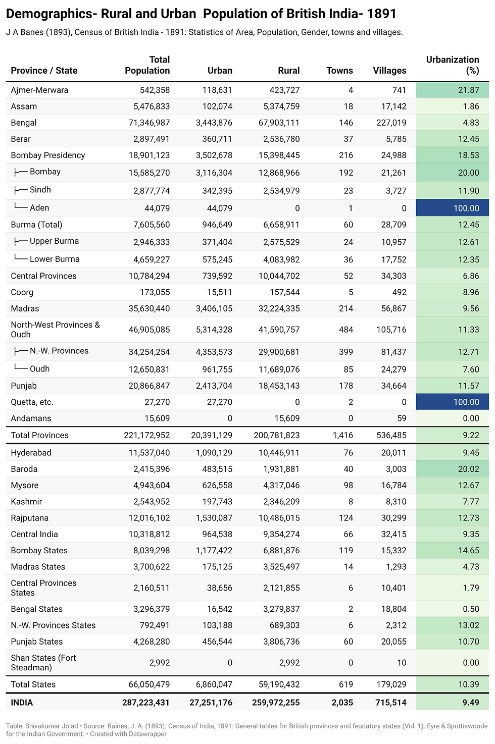
We can see the overwhelming rural concentration as a strength of the village system, which provided most people's economic, social, and cultural needs through long-established customs and inherited social arrangements. 

For the vast majority of Indians, urban life remained distant and unfamiliar. The urban population was also diluted by the existence of many small settlements classified as towns for administrative or revenue purposes but lacking the economic and social characteristics usually associated with urban centres. 

Despite India remaining largely rural, the decade between 1881 and 1891 saw the rise of new urban centres linked to trade, industry, and better transport. At the same time, many older capitals and former provincial cities, such as Patna and Surat, either grew slowly or declined. 

In contrast, port and industrial cities expanded rapidly. Karachi and Rangoon were among the fastest-growing, with their populations increasing by 43 percent and 34 percent respectively. According to the census, these cities grew because of expanding British trade networks and their role as major centres for the movement and distribution of goods.

Industrial growth also helped many cities expand. Places such as Cawnpore (Kanpur) and Ahmedabad became important centres of both trade and manufacturing. In Cawnpore, industries like leather production grew rapidly because they supplied goods to the military and police. 

The expansion of railway networks and the growing movement of commercial capital further boosted these cities. As a result, new opportunities emerged for traders, professionals, and industrial workers, encouraging urban growth.

At the same time, many older towns that had relied on royal courts and traditional centres of political power found it difficult to adjust to the changing economy. Cities such as Bijapur and Murshidabad often declined as trade, investment, and economic activity shifted to newer commercial and industrial centres. 

As a result, the urban landscape of late nineteenth-century India was changing, with older court-based towns losing importance while modern cities driven by trade, industry, and transport networks continued to grow.

Table: Distribution of Towns and Villages by Province and State Agency

A Population Rooted to Its Place of Birth 

Census described the Indian population as being strongly tied to its place of origin, displaying what officials called an "adscription to the soil." In a predominantly agricultural society, most people remained closely attached to their ancestral villages and rarely moved far from where they were born. 

The census report suggested that migration was limited not only by economic conditions but also by social, linguistic, and cultural boundaries. For many villagers, moving beyond familiar regions meant crossing into areas with different languages, customs, and social networks, making long-distance migration uncommon.

The census figures highlight how limited migration was in India during this period. According to the 1891 Census, 96.6 percent of the population lived either in their birthplace or in a neighbouring district. Out of every 10,000 people counted, 9,038 were living in the district where they were born, while another 623 had moved only from a nearby district. This meant that only about 3.5 percent of the population had migrated from more distant parts of India or from outside the subcontinent.

As a result, what appeared as migration in the census records often reflected marriage-related movement rather than economic migration. Census officials referred to this pattern as an “interchange of wives” between neighbouring communities.

This pattern was closely linked to the marriage customs of the time. Under the Brahmanic marriage system, people were expected to marry within their caste but not among close relatives. As a result, families often looked for marriage partners in nearby villages that belonged to the same social group, leading to a regular movement of women over short distances after marriage. While such movement appeared in migration statistics, it did not greatly change the overall picture of a largely settled and immobile population.

Strong evidence found that much of the movement between neighbouring districts was linked to marriage rather than economic migration. While the overall population recorded 958 females for every 1,000 males, people who had migrated from a neighbouring district showed a dramatically different pattern, with 1,370 females for every 1,000 males.

“…Then, again, the movement from the contiguous territory is not migration, in the ordinary sense. Instead of being the transfer of families, it is mainly the interchange of children in marriage a practice which obtains to a greater or less extent according to the predominance of the influence of Brahmanic prescription, with its strict observance of endogamy, as it is usually termed, within the caste or tribe and the accompanying prohibition of marriage within certain degrees of relationship, of which some are, according to western motions, rather remote.”

In Orissa, for example, the ratio among migrants from neighbouring districts reached 1,934 females for every 1,000 males. In contrast, Eastern Bengal, where Muslim marriage practices did not follow the same restrictions as the Brahmanic system, recorded a much lower ratio of 687 females per 1,000 males among contiguous migrants. These regional differences reinforced the census view that local migration was closely tied to marriage customs and the movement of women between nearby communities.

Internal economic migration also existed but was often temporary or seasonal in nature. Labourers travelled to work in Assam's tea plantations, the docks of Bombay and Calcutta, or seasonal agricultural harvests, but many returned to their home villages after completing their work. 

Movement between British-administered territories and the princely states was also found to be broadly balanced. It is also recorded that there is only a small net difference, with around 916,000 more people moving from British provinces to princely states than in the opposite direction. Given the size of the overall population, this was not considered a major demographic shift. 

Sex Ratios: Proportions and Discrepancies

Gender Imbalance in the 1891 Census

A striking imbalance between men and women in India was also noted. Unlike most European countries at the time, where women outnumbered men, India recorded significantly fewer women than men. Across the country, there were only 958 women for every 1,000 men, resulting in a female deficit of approximately 6.25 million. However, this pattern was far from uniform across the subcontinent.

A few provinces reported more women than men. Madras recorded 1,022 women for every 1,000 men, Bengal reported 1,006, and Upper Burma showed the highest ratio at 1,084. These regions stood in contrast to the broader national trend and represented some of the few areas where women outnumbered men. 

The shortage of women was most severe in the northern and north-western regions of the empire. Punjab recorded only 854 women for every 1,000 men, while Sindh had one of the lowest ratios at 831. Other areas with substantial female deficits included the North-West Provinces, where the ratio stood at 923, Rajputana at 891, and Kashmir at 879 women per 1,000 men. These regional differences reveal that the gender imbalance was unevenly distributed across India.

While some provinces maintained relatively balanced populations or even a female surplus, others experienced severe deficits. The census thus highlighted the considerable variation in demographic conditions across the Indian Empire at the close of the nineteenth century.

Why Were There Fewer Women?

The census looked into whether the shortage of 6.25 million women was entirely real or partly the result of undercounting. Census officials identified the concealment of women as an important factor, particularly in northern India. 

This undercounting was especially visible among girls and young women aged 10 to 20 years. Families were often reluctant to report unmarried daughters of marriageable age, while newly married women living in seclusion were frequently omitted from census schedules. 

The report also argued that the female deficit was partly real and linked to higher mortality among women. Although female infanticide had become less common by 1891, the neglect of girl children remained a concern. Sons were often given better food and quicker medical attention, while girls received less care and support during illness. 

High maternal mortality was another major factor. Early marriage, childbirth at a young age, repeated pregnancies, and the lack of trained medical assistance placed women at considerable risk. Unskilled midwifery and poor obstetric care, especially in rural areas, contributed to many deaths during childbirth. 

The census further suggested that the physical and emotional strain associated with puberty, marriage, and motherhood weakened women's health during these crucial years, adding to the overall gender imbalance.

Climate, Nutrition, and the Female Deficit

The census also suggested that climate and nutrition may have influenced the balance between men and women. Census officials observed that women appeared to survive in greater numbers in coastal and hill regions than in the hot and dry interior plains.

Nutrition was considered another important factor. In fertile and well-watered regions, where people had access to a more varied and reliable food supply, the gender balance tended to be more equal. 

However, in poorer areas with lower living standards and limited food resources, women were believed to be more vulnerable to disease, malnutrition, and the general "wear and tear of life."

Taken together, these observations led census officials to conclude that the shortage of women in India was not caused by a single factor. Rather, it resulted from a complex combination of environmental conditions, nutritional inequalities, and deeply rooted social practices that shaped women's lives and survival chances.

Challenges in Recording Age

The 1891 Census found that age data collected from the population was often highly inaccurate. A major reason given for this was that most people did not know their exact age. While a small educated section of society could sometimes refer to horoscopes or written records, the majority considered age unimportant once they reached adulthood.

As a result, many people estimated their ages rather than reporting them precisely. Census officials observed a strong preference for ages ending in multiples of five. Numbers such as 30, 40, 50, and 60 were reported far more frequently than expected, while 25 emerged as a particularly popular age. In contrast, ages immediately before or after these round numbers—such as 29 or 31—appeared far less often in the census records.

This pattern suggests that many respondents rounded their ages to familiar or convenient figures, making the age data less reliable and highlighting the difficulties faced by census officials in collecting accurate demographic information.

Table: Population by Age Group (India Total, 1891)

A Young Population with a Short Life Expectancy

Despite problems with age reporting, the 1891 Census clearly showed that India had a very young population. Children made up a much larger share of the population than was common in Europe at the time. One striking finding was that 94 percent of all unmarried females were below the age of 15. This reflected the widespread practice of early marriage.

Among girls aged 10 to 15, nearly half were already married, leaving very few unmarried women beyond puberty. This youthful population structure was sustained by a very high birth rate, estimated at nearly 48 births per 1,000 people. High fertility was necessary to maintain population growth in the face of heavy mortality.

At the same time, the census pointed to what officials described as a lack of "staying power" among the population. Compared to European countries, there were far fewer people aged 40 and above. The proportion of older adults was significantly lower than that found in European age distributions, suggesting that many people died relatively young. 

Life expectancy at birth was estimated at only 25 years for males and just under 26 years for females. In comparison, life expectancy in England was over 41 years for men and nearly 45 years for women. A major reason for this low average was the extremely high rate of infant mortality. Nearly 29 per cent of boys and 26 per cent of girls died during their first year of life. 

Children who survived infancy had much better chances of living longer, with life expectancy reaching its highest point around the age of six. Even then, boys could expect about 40 more years of life and girls about 37. The result was a society with a large number of children, relatively few elderly people, and generations succeeding one another much more rapidly than in Europe.

Measuring the "Value of Life" in India

The census went beyond simply counting people and attempted to measure life expectancy across the Indian Empire. Using detailed birth and death records from Madras City and selected communities in the North-West Provinces, census officials prepared life tables to estimate how long people could expect to live. 

These calculations, developed by actuary Mr Hardy, were based on the decade between 1881 and 1891, which was considered relatively normal and free from major famines or severe epidemics.

These figures indicate that life expectancy in India was substantially lower than in England, particularly during the most productive years of life. The difference was especially striking in infancy, where survival chances for Indian children were much lower than those of children born in England. High infant mortality played a major role in reducing the overall life expectancy of the Indian population.

Table: Life Expectancy for India and England & Wales

The low life expectancy recorded in the 1891 Census was largely the result of extremely high infant mortality. The data also reflected a common biological pattern seen in many populations: female infants had slightly better survival chances than male infants. However, the overall level of infant mortality in India was so high that it significantly reduced the average life expectancy of the entire population. 

According to census officials, several factors contributed to these deaths. Poor maternal and child healthcare, unskilled midwifery, and the absence of trained medical assistance during childbirth were identified as major causes, particularly in rural areas where access to professional healthcare was limited.

Table: Adjusted Infant Mortality Rates by Province (Life Tables) 

Source: Imperial Tables vol 2

For those who survived the dangers of infancy, the statistical outlook improved considerably. Census found that the expectation of further life reached its highest point around the age of six. At this stage, a male child could expect to live approximately 40 more years, while a female child could expect about 37 additional years. 

This suggests that although many children faced a high risk of death in their early years, those who survived beyond the age of five entered a relatively more secure phase of life. After this peak, life expectancy gradually declined due to diseases and general hardships of life. 

To maintain a population exposed to such high levels of mortality, birth rates had to remain exceptionally high. Census estimates suggested that a birth rate of nearly 48 per 1,000 population was necessary simply to sustain the population. 

This was required to offset an average death rate of about 41 per 1,000. Even in years unaffected by major famines or epidemics, the population depended on a very large number of births to offset the constant losses from ordinary mortality. Population growth, therefore, relied on a continuous process of demographic replenishment.

This combination of high birth rates and high death rates meant that generations succeeded one another much more rapidly than in Europe. The census identified a notable shortage of people aged 40 and above, with the proportion of older adults more than 5 per cent lower than that recorded in European age tables. 

This limited "staying power" of the population reflected the fact that many people died relatively young. By the age of 50, the survival prospects of an Indian male were estimated to be roughly one-third lower than those of an Englishman of the same age. The census analysis also highlighted several factors that contributed to these mortality patterns. 

Living standards for much of the population were often close to subsistence levels, even though the population continued to grow during normal years. Early marriage, premature cohabitation, repeated childbearing, poor maternal health, and inadequate medical care all contributed to elevated mortality. 

The report further pointed to limited knowledge of hygiene and the crowded conditions found in some rural areas as factors that worsened health outcomes. It also observed that female survival tended to be higher in coastal and hill regions than in the hot and dry interior plains.

Taken together, the actuarial analysis presented in the 1891 Census depicts an empire shaped by intense demographic pressures. Although the population was capable of growing during periods of relative stability and prosperity, this growth was sustained only through a continuous cycle of high fertility and high mortality. 

The "Value of Life" in late nineteenth-century India was therefore defined not only by a comparatively short lifespan but also by the enormous reproductive effort required to maintain the population in the face of persistent and widespread mortality.

Marriage and Widowhood: A Social Reality

Census identified the near universality of marriage as one of the defining features of Indian society. For much of the population, particularly among Brahmanic communities, marriage was viewed not merely as a personal choice but as a religious and social obligation. Producing a male heir was considered essential for performing funeral rites and ensuring continuity of the family line. 

Therefore, marriage often took place at a very young age. Census data showed that 17 percent of all girls below the age of 15 were already married (1,702 per 10,000), a pattern that had few parallels in contemporary Europe. By the time women reached the main reproductive ages of 15 to 40 years, about 84 percent were married, compared to roughly half of women in Western countries.

The strong emphasis on early marriage, together with the often large age gap between husbands and wives, contributed to the high number of widows in India. Census analysis showed that India had about 36 percent more widowers than were typically found in Europe, but the number of widows was much higher—around 122 percent more than in European countries. 

One of the main reasons for this imbalance was the widespread restriction on widow remarriage in many Brahmanic communities. Under these customs, even a girl who had been married or betrothed in childhood could be required to remain a widow for the rest of her life if her husband died.

The census observed that these customs were not limited to the highest castes. Over time, many lower-caste groups adopted practices such as child marriage and the discouragement of widow remarriage because they were seen as signs of higher social status and respectability. As a result, customs once associated mainly with elite groups gradually spread across wider sections of society.

These practices had important demographic effects. While widowers were often able to remarry and return to married life, widows faced strict social restrictions and had far fewer opportunities to do so. Consequently, widows made up a large share of the female population. According to the census, 17.6 percent of all women in India were widows—more than twice the proportion found in most European countries at the time.

Conclusion

The 1891 Census provides a detailed picture of Indian society at the end of the nineteenth century. It shows that India was overwhelmingly rural, with more than nine out of every ten people living in villages. Village communities remained the centre of economic, social, and cultural life, and most people depended directly on agriculture for their livelihood. Although some towns and cities existed, urban life remained limited for the vast majority of the population.

At the same time, the census recorded important economic changes. New cities such as Karachi, Rangoon, Cawnpore, and Ahmedabad grew because of expanding trade, industries, and railway networks. These centres created new opportunities for merchants, workers, and professionals. 

However, many older towns that had depended on royal courts and traditional political power, such as Surat, Patna, Bijapur, and Murshidabad, either stagnated or declined as economic activity shifted towards modern commercial centres.

The census also portrayed India as a society with very low levels of migration. Much of the movement recorded in the census was related to marriage, particularly the movement of women between neighbouring villages and districts. Social customs, language differences, and strong local ties continued to keep most people closely connected to their native communities.

Finally, the census highlighted several important social challenges, including a shortage of women, widespread child marriage, a large number of widows, high infant mortality, and low life expectancy. These patterns reflected the combined influence of social customs, poor healthcare, and difficult living conditions. Taken together, the findings of the 1891 Census reveal an India that was beginning to experience economic and urban change, but one where traditional social structures and rural life continued to shape the lives of most people.

(Authors: Umesh Bedkute is a an independent researcher, data analyst and data journalist working at the intersection of policy, education and governance. 

Dr. Shivakumar Jolad works as Associate Professor (Public Policy), and is the Chair of Center for Legislative Education and Research and Director India State Stories, FLAME University, Pune

Umesh contributed to research and primary writing;  Shivakumar contributed to conceptualization, research and editing)

Source:

Baines, J. A. (1893). General Report on the Census of India, 1891. London.